EchoDyne's Counter-UAV Radars

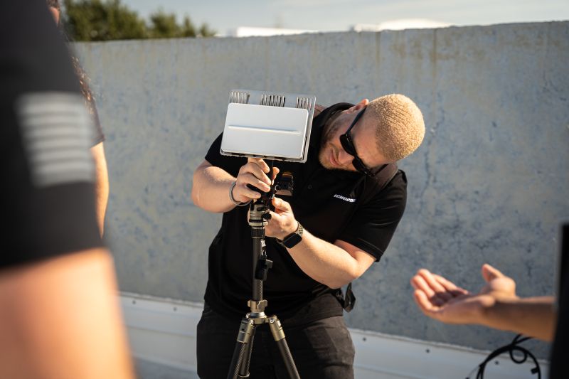
This morning the LinkedIn brought an interesting photo of a small radar for drones detection:

The value of Echodyne radars cannot be understated. A compact unit, this system capable of accurately detecting, classifying, and tracking aircraft in its immediate vicinity. This system is optimal for teams needing a portable unit to watch over specific locations like public events.

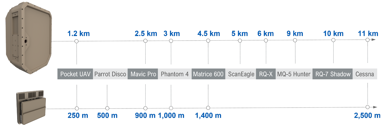
It is developed by the Echodyne company. This small, tablet-sized radar provides precise 3D coordinates with fast update rate, has impressive characteristics, the promised easy-to-use APIs, flexible embedded software, and multiple data output options. It also has quite impressive capability for tracking drones at short ranges:

Echodyne radar tracking ranges for air targets

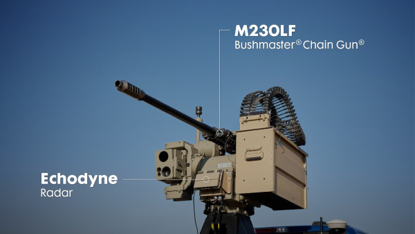
It also can be used even for weapon control at last stages:

EchoGuard radar control the gun

The radio wave propagation within the surface duct and the sinking of the Russian Black Sea Fleet cruiser Moskva

Accordingly to the recent publication in Forbes, in days and weeks after a Ukrainian navy anti-ship missile battery sank the Russian Black Sea Fleet cruiser Moskva on April 13, a lot of rumors circulated. Many of them attempted to explain how the Ukrainian navy, which does not have big ships or aircraft, could defeat a navy with lots of big and heavily - armed - vessels and planes. Some of the rumors hinged on the assumption that the Ukrainians required foreign help in order to strike Moskva.

But according to the cited in Forbes an eyebrow-raising new story in Ukrainska Pravda, the Neptune battery — a quad launcher and its associated radar — found and hit Moskva mostly on its own. The assistance the battery did receive from an atmospheric phenomenon called “temperature inversion” created a kind of channel for radar waves that allowed them to travel over the curve of the horizon and back.

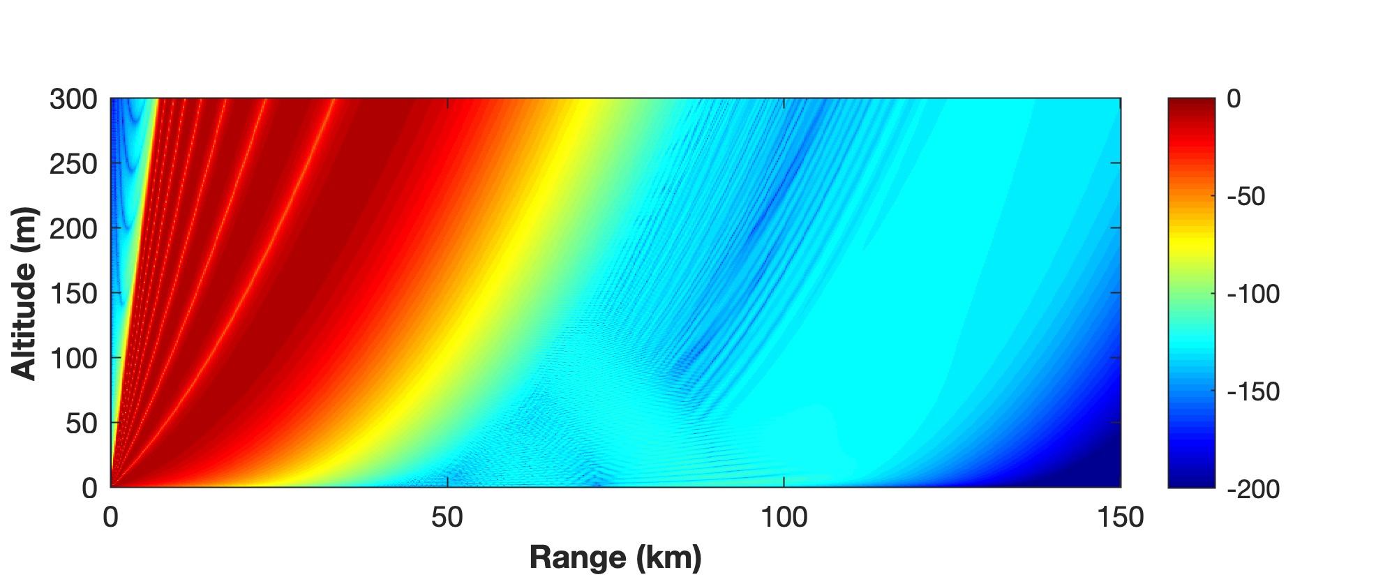
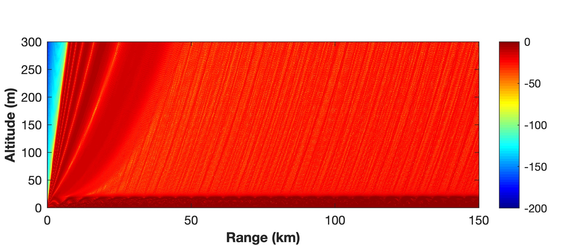
Using the PETOOL Matlab package it is quite easy to visualize the standard situation of radar signals propagation above the sea surface. In standard situation that most often takes place during the spring in the Black Sea regions, the propagation factor (it is the factor that shows the value of attenuation of the transmitted signal that approaches a specific location and reflected back to the radar) is shown in Figure 1 using the logarithmic (decibels) scale.

Figure 1. The radio waves propagation factor in case of radar antenna installed at the height 3 m in a standard atmospheric conditions.)

Clear, that the strong attenuation (around 150 dB, 15 orders of power loss) of the signals from the ship that was at that time well below the radio-horizon, at the 120 km distance from the radar position, did not give a possibility to detect and track it, making impossible the operation of the Neptune battery.

But in the case of mentioned above “temperature inversion” the profile of the refractive index of atmosphere has very specific shape that radio-engineers called as the “surface duct”. In that case radio waves are propagating as in a waveguide for much longer distances. In this case the propagation factor looks quite different from the case of standard atmospheric conditions - see Figure 2.

Figure 2. The radio waves propagation factor in case of a radar antenna installed at the height 3 m in a "surface duct" conditions (the height of the inverse layer in this case equals to 20 m).

We see that inside the surface duct radar signal propagates between surface and upper limit of the inversion layer practically without serious attenuation. In such a case the huge ship at the distance of 120 km, well behind the radio-horizon, can be easily detected and destroyed using guided missiles.

news

Today these pages have been moved finally from the personal pages location at TU Delft (homepage.tudelft.nl/v0e47), where it existed for more that 14 years, to the new github site…

With a hope that it has new home for a long time…

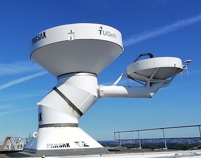
PARSAX radar

Colouring of the mixture of 2D signals

Sometimes it is necessary to make an image of the mixture 2D data using different PGB pallets for every component.
For example, let create three 2D functions:

for (ix=1:100), 
    for (iy=1:100), 
        z(ix,iy)= exp(-(ix-30).^2./500).*exp(-(iy-30).^2./500);
        z1(ix,iy)=exp(-(ix-50).^2./300).*exp(-(iy-50).^2./900);
        z2(ix,iy)=exp(-(ix-80).^2./350).*exp(-(iy-80).^2./50);
    end;
end;

We can easily make an image of the resulting mixture of these function:

figure;imagesc(z+z1+z2)
title('Image of the signals'' sum')

As result we will have the image of the mixture as a sum of all functions:
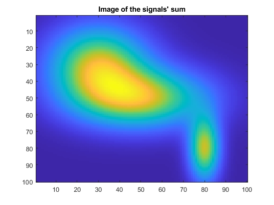
Image of the mixture as a sum

We can see the total behaviour of the functions sum but not every component. To keep that information is possible using by changing colour palettes for every component of the mixture. For example, we can use the blue pallete for the signal z, the grey palette for the signal z1, and yellow - - for the signal z2. For these we have to do following:

q(:,:,1)=zeros(100,100);q(:,:,2)=zeros(100,100);
q(:,:,3)=z;

q1(:,:,1)=z1;q1(:,:,2)=z1;q1(:,:,3)=z1;

q12(:,:,1)=z2;
q12(:,:,2)=z2;
q12(:,:,3)=zeros(100,100);

figure;imagesc(q+q1+q12)
title('black-based signals colouring: the sum')

The result will look as follow:
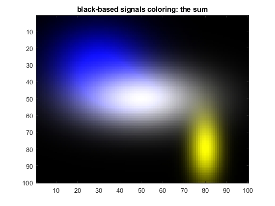
Image of the coloured mixture as signals with zeros as black

Now we can see not only 2D variability of the mixture of functions, but clear recognize the values of every component. What still can be improved is to apply the negative grey palette, when the minimum is represented as white and maximum - as the black colour. Such inverted palette is much more suitable for printing and for insertion in publications.
It can be done using following codes:

z21=(max(max(z))-z)./max(max(max(z))-z);
q21(:,:,1)=z21;q21(:,:,2)=z21;q21(:,:,3)=z21;

z22=(max(max(z1))-z1)./max(max(max(z1))-z1);
q22(:,:,1)=ones(100,100);q22(:,:,2)=z22;q22(:,:,3)=z22;

z23=(max(max(z2))-z2)./max(max(max(z2))-z2);
q23(:,:,1)=z23; q23(:,:,2)=z23; q23(:,:,3)=ones(100,100);

Q=(q21+q22+q23);
Q=Q./max(max(Q));

figure;imagesc(Q)
title('white-based signals colouring: the sum with normalization')

To extend every component visualization to the full scale of specific palette, we did the normalization of every function. As soon as the sum of functions cam be greater than 1 within the RGB components of the colours representation, the final sum Q was also normalized using its maximum value (in general, the minimum value also has to be taken into account for such normalization).
The resulting image looks as follow:
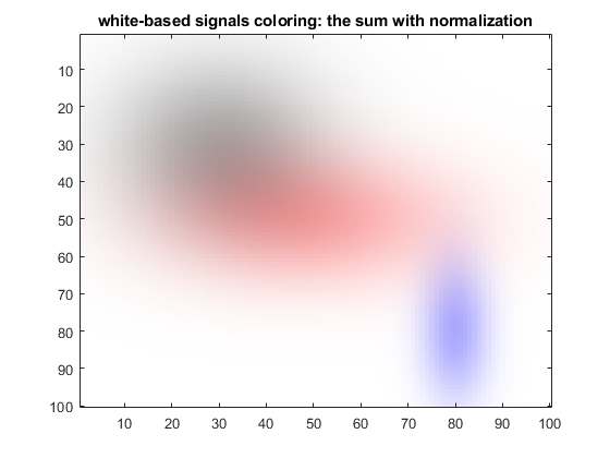
Image of the coloured mixture as a sum signals with zeros as white

It can be seen that if to use for such representation the sum of RGB codes of signal components, the dynamic range of colour image is seriously reduced - red becomes light red, blue - light blue, black-dark grey - not much dark. It is defined by the necessity of the total scaling of the sum of individual RGB scales of components. To overcome such reduction of the final image RGB scale, instead of the sum can be used piecewise product of RGB coded components:

Q1=(q21.*q22.*q23);

figure;imagesc(Q1)
title('white-based signals colouring: the product')
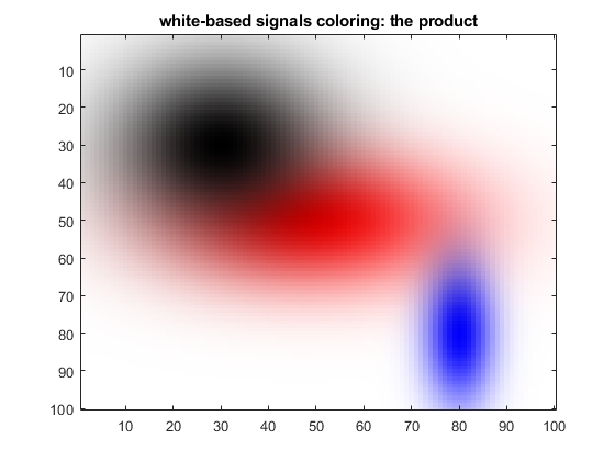
Image of the coloured mixture as a signals product with zeros as white

In this case the final scaling is not necessary, and the dynamic range of the selected colours is much wider…