Accordingly to the recent publication in Forbes, in days and weeks after a Ukrainian navy anti-ship missile battery sank the Russian Black Sea Fleet cruiser Moskva on April 13, a lot of rumors circulated. Many of them attempted to explain how the Ukrainian navy, which does not have big ships or aircraft, could defeat a navy with lots of big and heavily - armed - vessels and planes. Some of the rumors hinged on the assumption that the Ukrainians required foreign help in order to strike Moskva.
But according to the cited in Forbes an eyebrow-raising new story in Ukrainska Pravda, the Neptune battery — a quad launcher and its associated radar — found and hit Moskva mostly on its own. The assistance the battery did receive from an atmospheric phenomenon called “temperature inversion” created a kind of channel for radar waves that allowed them to travel over the curve of the horizon and back.
Using the PETOOL Matlab package it is quite easy to visualize the standard situation of radar signals propagation above the sea surface. In standard situation that most often takes place during the spring in the Black Sea regions, the propagation factor (it is the factor that shows the value of attenuation of the transmitted signal that approaches a specific location and reflected back to the radar) is shown in Figure 1 using the logarithmic (decibels) scale.
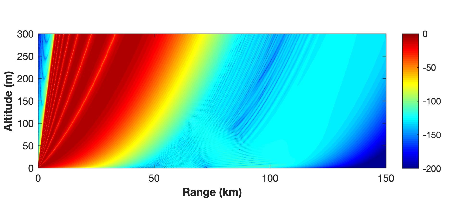
Clear, that the strong attenuation (around 150 dB, 15 orders of power loss) of the signals from the ship that was at that time well below the radio-horizon, at the 120 km distance from the radar position, did not give a possibility to detect and track it, making impossible the operation of the Neptune battery.
But in the case of mentioned above “temperature inversion” the profile of the refractive index of atmosphere has very specific shape that radio-engineers called as the “surface duct”. In that case radio waves are propagating as in a waveguide for much longer distances. In this case the propagation factor looks quite different from the case of standard atmospheric conditions - see Figure 2.
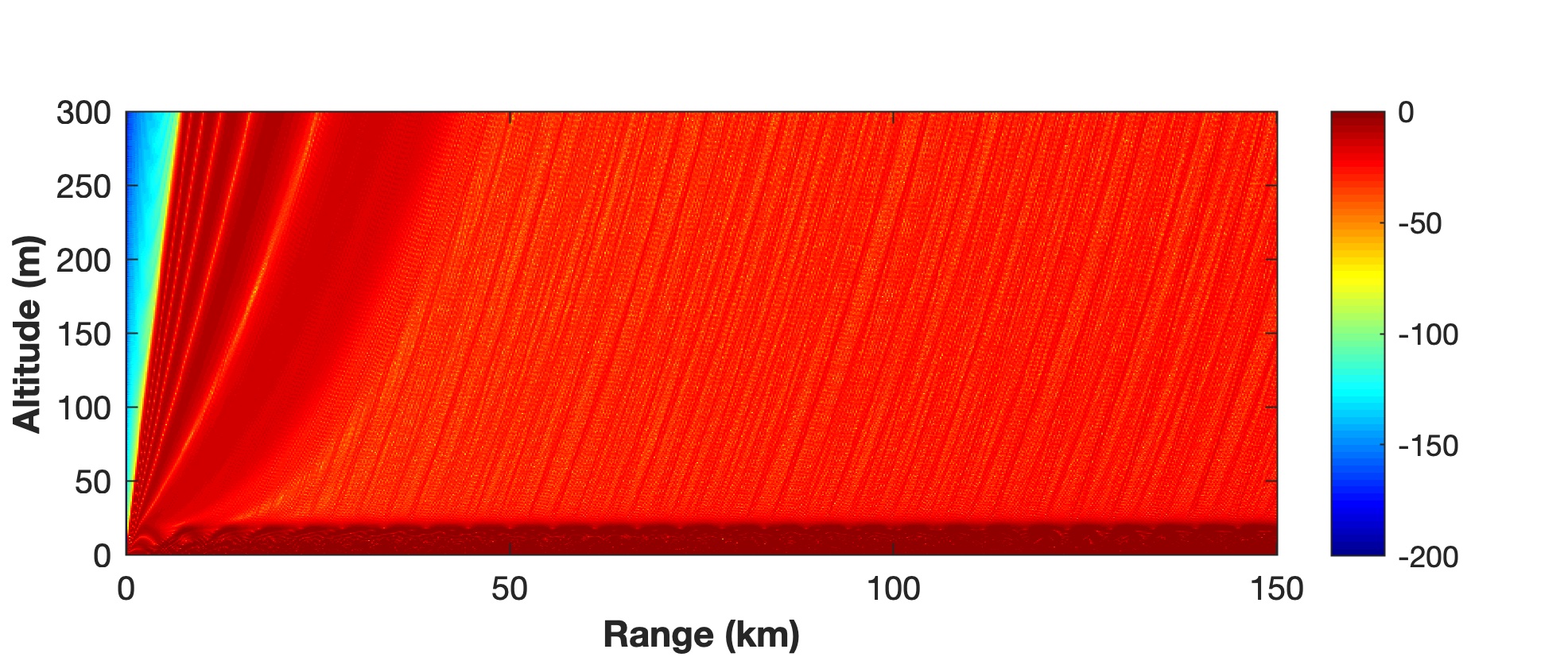
We see that inside the surface duct radar signal propagates between surface and upper limit of the inversion layer practically without serious attenuation. In such a case the huge ship at the distance of 120 km, well behind the radio-horizon, can be easily detected and destroyed using guided missiles.